Summary
This text presents hydrogenation as a method of laboratory and industrial synthesis. The first part provides an introduction to the theory of catalysis. Then we will focus on the issue of obtaining reliable kinetic data in laboratory hydrogenation in the liquid phase. The next chapter is devoted to methods of gas phase hydrogenation research. The last chapter is devoted to the interpretation of kinetic data obtained during gas phase hydrogenation.
1. Theory of catalytic action
Almost all chemical industries are built on catalytic processes. We distinguish homogeneous catalysis, where the catalyst is dissolved in the liquid phase – an example is the production of the vast majority of polymers; and catalysis heterogeneous, where the catalyst is in the form of tablets through which a stream of reactants passes or is optionally in the form of a powder dispersed in a liquid or gaseous phase. This text will focus on heterogeneous catalytic hydrogenation.
While industrial processes are generally perfectly mastered, not much is known about the actual course of catalytic action. One of my professors once said, “Until recently, everyone who had a hole in their ass came up with their theory of catalysis. Pay God, it’s over. ” He wasn’t quite right. Chemical literature is growing unstoppably, we are flooded with new knowledge every day, so it is legitimate to look for a way to sort this knowledge. The search for a Systema Naturæ (according to Carl von Linnaeus‘ terminology, 1735) is therefore a legitimate effort.
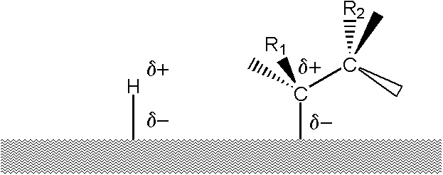
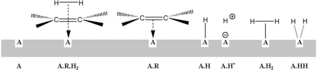
So let’s look at the most common ideas about the mechanism of heterogeneous hydrogenation. The catalytic surface usually consists of the area of metal atoms in a triangular clip. Multiplet theory states that the center of catalytic activity is not individual metal atoms, but whole groups of atoms:
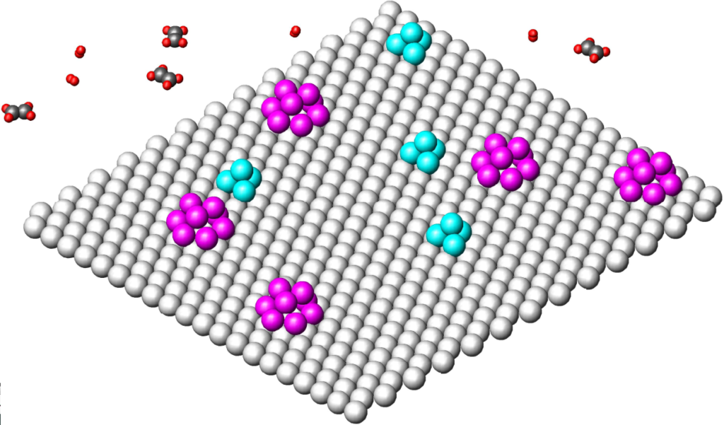
For reasons given by kinetic findings (see below: zero order for both components), it is considered that there is not only one type of multiplet on the surface, but at least two types of multiplets, one of which is only able to activate hydrogen and the other only olefin; this is the so-called „two-surface theory.“ Our image represents such a surface with multiplets of two colors, two kinds. The ethylene and hydrogen molecules (above) are plotted with the following interatomic distances (1Å = 10-10m): H-H 0.56; C = C 1.33 (in other figures also: C-C 1.54); C-H 1.05. We will display metal atoms, on the same scale, with an interatomic metal-to-metal distance of 2.6 which is a kind of mean value for metals capable of hydrogenation.
To the previous picture: let’s say that purple multiplets are able to activate only olefin and those light blue only hydrogen. The activated molecules then need to be brought into contact with each other, which is impossible from the point of view. Unless the Montpellier professor (Pierre Brun: Catalyse et catalyseurs en chimie organique, Masson 1970) was right, who judged that by simply approaching the surface, the reactants gain a magical power that allows them to react in space outside the catalytic surface.
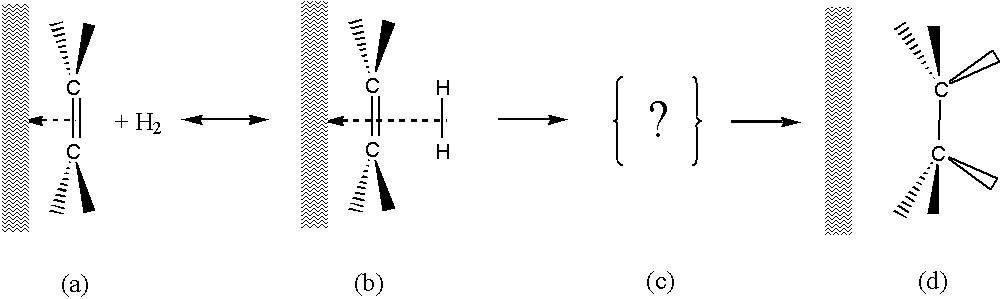
In practically every textbook of organic chemistry we find the so-called „semi-hydrogenated state theory“ (Horiuti and Polanyi, 1934). This is how Wikipedia.org presents it under the term „Hydrogenation“:
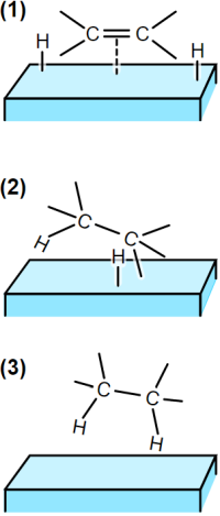
Legend:
(1) The reactants are adsorbed on the catalyst surface and H2 dissociates.
(2) An H atom bonds to one C atom. The other C atom is still attached to the surface.
(3) A second C atom bonds to an H atom. The molecule leaves the surface.
The theory of the semi-hydrogenated state is intended to explain why isomerization often occurs during the hydrogenation of olefins: in the reversible reaction from (2) to (1), according to this theory, hydrogen other than that previously bound should be cleaved.
Another presentation of the same theory:
We have at least seven reasons (N° 1 to N° 7) to believe that this theory is incorrect.
First (Objection # 1):
same as in the two-surface theory – can fragments of molecules travel across the surface at all, as this mechanism requires?
The principle of microscopic reversibility says that if the reaction runs in one direction over certain intermediates, then the reaction in the opposite direction will run over the same intermediates. Of course, in the case of hydrogenation, it is necessary to raise the temperature a lot to induce the opposite reaction, but why should hydrogen travel far to the surface after cleavage?
Second (Objection # 2):
It has been observed that in the hydrogenation of 1-olefins in the liquid phase, by increasing the hydrogen pressure, it is possible to reach a state where the reaction is zero order with respect to both components, i.e. both the olefin concentration and the hydrogen pressure. As we will show below, with competitive adsorption of both components on the surface, this is ruled out.
Third:
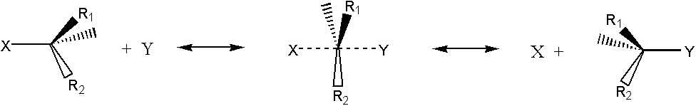
Organic chemists learn that there is only one transition state between the initial and final state of a chemical reaction, and this is as symmetrical as possible (Objection # 3). An example is the Walden reaction, ie the exchange of halogen X for halogen Y. If the substituents on carbon are different, the molecule exhibits optical rotation, inversing the reaction, demonstrating the approach of halogen Y on one side and the cleavage of halogen X on the other:
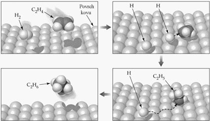
In our opinion, an analogous mechanism is well possible in the case of hydrogenation:
Legend:
(a) Olefin is adsorbed on a metal surface – a strong chemical bond.
(b) Hydrogen is adsorbed in the second layer – physical to chemical bond.
(c) A transient state in which the bond of the olefin to the surface weakens and at the same time the bond with the hydrogen atoms is strengthened. Substituents on the carbons deflect towards the catalytic surface, which can prematurely weaken the olefin bond to the surface. Therefore, the hydrogenation of 1-olefins and a double bond with two substituents takes place, while the hydrogenation of tri- and tetra-substituted double bonds is excluded.
(d) The saturated molecule leaves the surface.
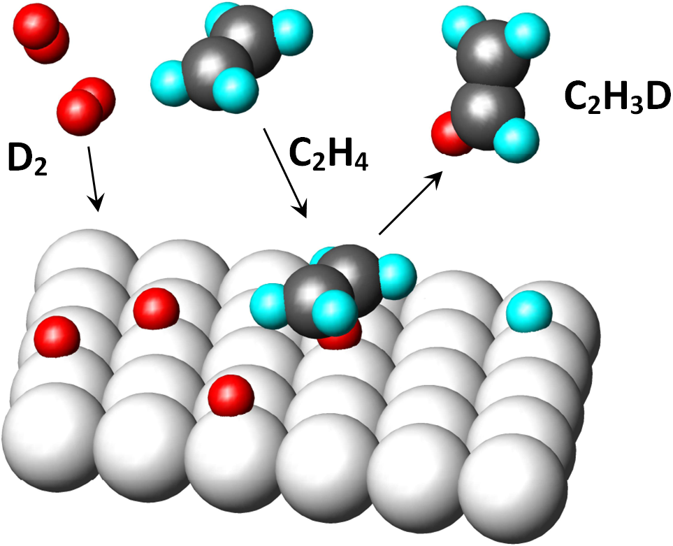
Space filling model:
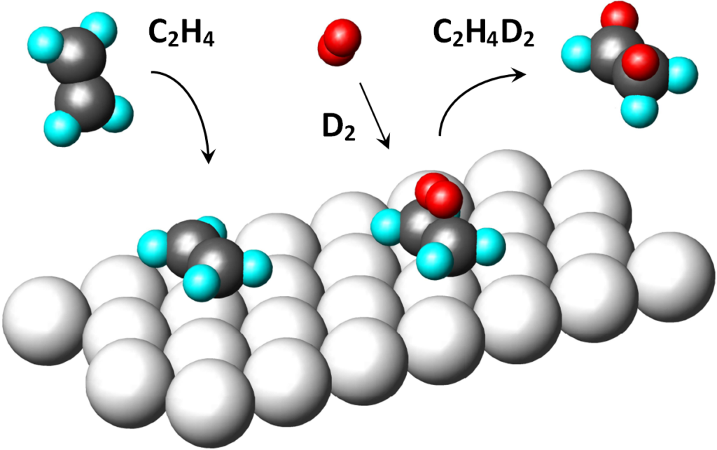
In the picture, the original hydrogens are cyan, the newly bonded hydrogens (D2) are red. It is a cis-addition of a whole molecule of hydrogen.
It was observed that e.g. on a platinum catalyst, the hydrogenation of mixtures of H2 + D2 molecules produces a product which contains either none or two deuterium atoms. This observation is difficult to reconcile with the theory of the semi-hydrogenated state (Objection # 4).
We will return briefly to the previous theory, to the theory of multiplets. This was based on observations of benzene / cyclohexane conversion. This reaction is catalyzed only by metals whose surface forms a triangular structure with a distance between adjacent atoms between 2.40 and 2.77 Å. Metals with distances outside this range or with a different surface geometry are inactive. A hexagon representing six carbons can then be nicely drawn into such a structure:
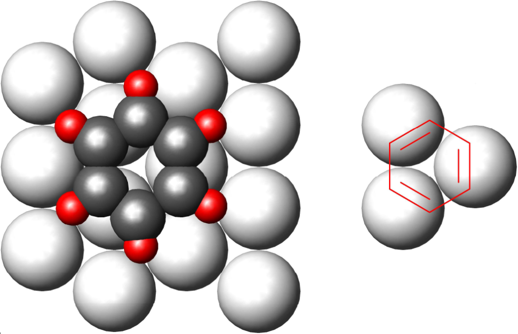
If we look at the benzene nucleus as a grouping of three double bonds, then only the rule is confirmed that only one metal atom is sufficient for the hydrogenation of one double bond.
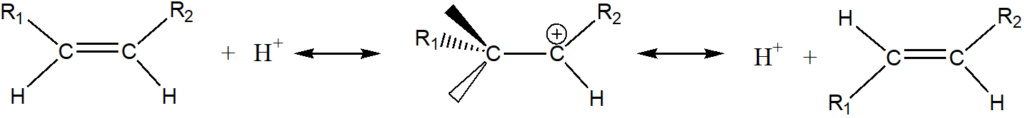
We will now turn to isomerization. The isomerization can be an isotope exchange reaction, cis / trans isomerization or a double bond shift in the carbon chain. In a homogeneous environment, isomerization is a reversible reaction catalyzed by a hydrogen cation:
In the case of a heterogeneous reaction on metal surfaces in the presence of hydrogen, we assume that the isomerization is a reaction independent of hydrogenation, catalyzed – similar to a homogeneous environment – by protonic hydrogen. The presence of protonic hydrogen on the surface of the catalyst is at least highly probable. Let us recall, for example, the fact that hydrogen dissolved in a metal travels under the influence of an electric current, which is considered to be evidence of its presence in a „metallic“, ie protonic, form. The isomerization reactions can then be carried out with an intermediate of the type
Why is this not a semi-hydrogenated state? It would be about an electrophilic addition, where the C = C double bond is a nucleophilic agent. Examples of double bond reduction with reducing agents, i.e. „ionic hydrogenation“ or „transfer hydrogenation“, exist. In catalytic hydrogenation, however, this would require heterolytic cleavage of the hydrogen molecule (H+, H–), which is quite unthinkable on the surface formed by single metal atoms – let us recall in this context the terms hydrogen electrode, Nernst’s equation. but at a time when we attribute a positive charge to the atomic hydrogen bound to the catalyst surface, the theory of the semihydrogenated state falls apart (Objection # 5). But beware: this is true for homogeneous surfaces made of a single metal; in the case of a surface modified with another metal, this may not be the case, as Adams found with an iron-modified platinum catalyst a hundred years ago.
In addition, in the case of simple olefins (especially on Pt), hydrogenation in the liquid phase is syn-addition, thus producing a cis- product, while isomerization of the intermediate, as occurs during ionic hydrogenation, leads to a trans- product (Objection # 6).
Space filling model of isomerization:
The total amount of protonic hydrogen on the catalyst surface is probably related to the ability of the individual metals to dissolve hydrogen. Extreme is palladium, which is capable of dissolving 350-850 times more hydrogen than its own volume; a solid solution of hydrogen in palladium with a composition of Pd2H is even considered to be a defined compound. In contrast, in platinum it dissolves at normal temperatures and pressures on the order of only 10-7 cm3 H2 / cm3 Pt. There is a clear connection with the fact that isomerization reactions (as well as hydrolytic reactions) take place on platinum only to a small extent, on palladium usually to a large extent. In one study of hydrogenation at the expense of hydrogen dissolved in a catalyst, it was found that in this way more isomers are always formed (double bond migration) than in conventional hydrogenation under hydrogen on the same catalyst. According to those authors, on the osmium, iridium, platinum, ruthenium and rhodium blacks (black – metal oxide, reduced in situ) the strongly adsorbed form of hydrogen, ie atomic hydrogen, participates in the displacement of the double bond, while in hydrogenation the weakly adsorbed form, ie molecular hydrogen (# 7a).
It has been found that if the metal is dehydrogenated prior to hydrogenation of the olefin, it loses its isomerizing ability. The nickel catalyst on which 1-octin was previously hydrogenated loses the ability to isomerize 1-hexene, while its ability to hydrogenate this olefin remains unchanged (# 7b).
Isomerization is an equilibrium reaction. In cis/trans isomerization, the steric effect is mainly applied, so the equilibrium is markedly towards the trans-. The direction of double bond migration is in turn given by the polarization of the double bond by the induction effect; in the case of hydrogen transfer to another place in the carbon chain, the biblical „He who has little, it will be taken“ (Matthew 25:29) applies. However, when interpreting the experimental data, it should be borne in mind that isomerization is an equilibrium reaction, so there is also isomerization of the double bond from the branch point to a straight section. The isomeric olefin can then be stabilized by direct bonding to the catalytic surface and subsequently hydrogenated. Tri-substituted olefinic compounds which fail to hydrogenate on platinum can therefore be hydrogenated on palladium with its ability to isomerize, optionally on a metal supported on an acidic alumina support (γ-Al2O3) or in a mixture with alumina.
Kinetic model according to Langmuir and Hinshelwood
In the rate equations of homogeneous reactions, concentrations usually act as activities. For surface reactions, Hinshelwood defines activity as the ratio of the surface active sites occupied by the respective reactant to the total number of surface active sites. Adsorption on the surface is competitive and proceeds according to the Langmuir adsorption isotherm. Assume, for example, that the following adsorption complexes are present on the surface:
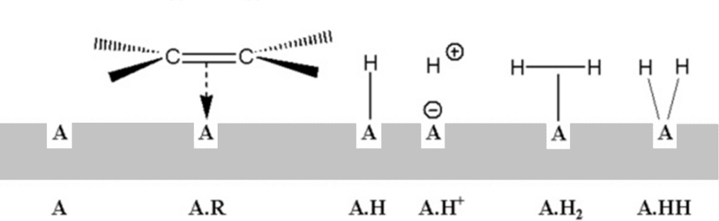
Langmuir balance, expressed first graphically and then by the equation:
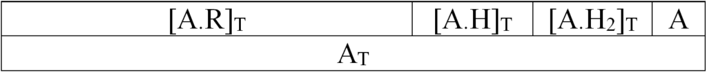
[A]T = [A] + [A.R]T + [A.H]T + [A.H2]T [1.1]
where:
[A]T total number of active surface sites
[A] unoccupied active seats
[A.R]T active sites occupied by olefin
[A.H]T active sites occupied by atomic hydrogen (A.H, A.H+)
[A.H2]T active sites occupied by molecular hydrogen (A.H2, A.HH)
An adsorption equilibrium constant can be defined for each adsorbed component:
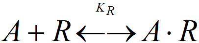
KR = [A.R]T/([A]·c)
where c is the activity (concentration) of olefin in solution
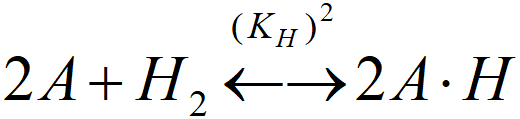
(KH)2 = [A.H]T2·/([A]2·PS)
where PS is the activity of hydrogen (its partial pressure at the catalyst surface, see next chapter)
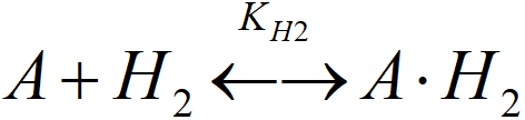
KH2 = [A.H2]T/([A]·PS)
Substituting into the initial balance equation we get
[A]T = [A] + [A]·KR·c + [A]·KH·PS0.5 + [A]·KH2·PS
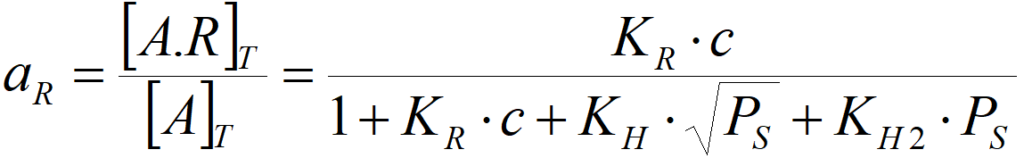
The olefin activity on the catalytic surface then amounts to
and similarly, for atomic hydrogen,
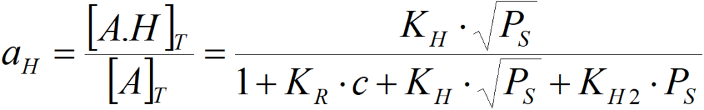
If virtually all active centers of the surface are coated with olefin,
ie KR·c >> 1 + KH·PS0.5 + KH2·PS,
then aR = 1 and further increasing the concentration practically does not change the activity, i.e. the reaction is zero order to the olefin. The activity against hydrogen is then (for atomic hydrogen) aH = KH·PS0.5/(KR·c) (where 1/KR·c is practically constant in this case) or the order of reaction against hydrogen will be non-zero. Similarly, if the surface is coated with hydrogen and the olefin is deficient, then the order of reaction with hydrogen will be zero, but the order with respect to olefin cannot be zero. In the case of competitive adsorption of two reactants, the order of reaction cannot be zero at the same time for both.
Thus, if a zero order of reaction with respect to both reactants was observed during the hydrogenation of olefins at higher pressure, this is not compatible with the theory of the semi-hydrogenated state.
Kinetic model of bilayer adsorption
We have tacitly accepted various simplifications in the Langmuir and Hinshelwood rate equation. Thus, we consider the number of active sites of the surface to be constant, independent of the degree of surface occupancy by individual adsorbed substances, and we consider all active centers to be equal. However, these and other simplifications do not affect the general validity of our conclusions.
We will now extend Hinshelwood’s theory to two-layer adsorption. We consider the following surface complexes:
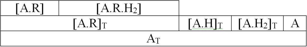
Graphic representation of the balance of both layers:
We have already solved the balance of the first layer. We assume that the adsorption of hydrogen in the second layer does not change the equilibrium in the first layer. Balance of the second (upper) layer:
[A.R]T = [A.R] + [A.R.H2]
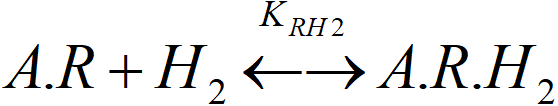
KRH2 = [A.R.H2]/([A.R]T·PS)
The surface concentration of the „two-layer“ complex A.R.H2 will be
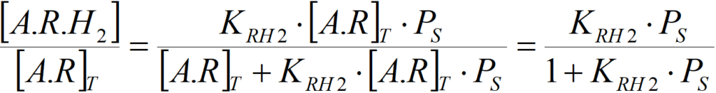
By multiplying the left and right sides of this equation by the above equation for aR = [A.R]T/[A]T we get
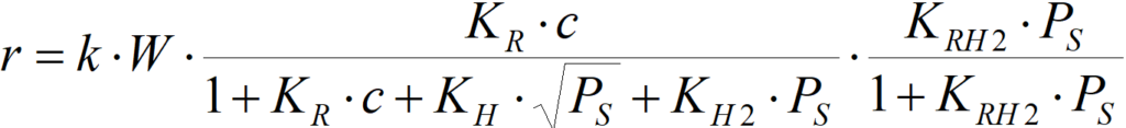
W is the amount of catalyst
k is the rate constant; it also includes the number of active centers AT per unit amount of catalyst W.
The equation must be understood as semi-quantitative – a lot of simplification was adopted in its derivation. However, provided that
KR·c >> 1+KH·PS0.5+KH2·PS and KRH2·PS >> 1, then
r = k·W [1.6]
that is: a zero order for both reactants, in a certain range of concentrations of reactants, is possible.
We conclude that, from a kinetic point of view, our theory of a two-layer activated complex also satisfies. For this reason, we recommend approaching the generally accepted „semi-hydrogenated state theory“ disapprovingly.
Other functional groups
Before leaving the theoretical part devoted to catalytic action, we return to the role of hydrogen bound directly to the catalytic surface. If our proposed model of catalytic hydrogenation of olefinic compounds excludes the direct participation of atomic hydrogen, including hydrogen dissolved in the metal mass, then it should be emphasized that for other functional groups, often strongly polarized, it will be different. An example of such a hydrogenation, which is difficult to imagine without the participation of protic hydrogen, is the hydrogenation of a benzaldehyde / dimethylamine mixture to give dimethylbenzylamine. On platinum the reaction gives a yield of about 90%, but on rhodium or palladium the selectivity is above 99%:
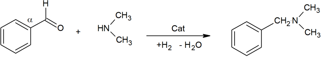
Here it appears that before the cleavage of water – the formation of the Shiff base, which is then further hydrogenated, an ammonium complex of surface atomic hydrogen with an amine is formed, i.e. protic hydrogen is catalytically involved directly in the main reaction.
As we have already mentioned in other contexts, in the hydrogenation of acetylenic compounds, i.e. the triple bond between carbons, surface hydrogen is directly consumed. On platinum, this reaction runs very slowly throughout the presence of the triple bond, but then the reaction rate increases sharply and the hydrogenation of the double bond takes place in a short time.
In conclusion, we reiterate that the ideas about the mechanism of heterogeneous catalysis are highly uncertain. In contrast, Hinshelwood’s theory of surface activities seems to be reliable.
2. Hydrogenation in the liquid phase
The problem of homogeneity of the reaction mixture
Hydrogenation of benzonitrile leads to benzylamine,
C6H5CN + 2H2 → C6H5CH2NH2
This industrial process also provides, to a small extent, dibenzylamine as a by-product. The market sometimes requires the production of dibenzylamine in larger quantities. A suitable method is the synthesis based on benzaldehyde and benzylamine:
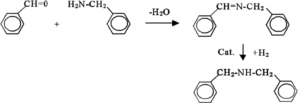
The Shiff-type intermediate is formed spontaneously by the separation of the aqueous phase, which, however, causes a catastrophically low yield (60%) of the final product. However, if the water is removed before the actual hydrogenation, the yield will increase to 98%. The generalization of this observation is that the formation of two liquid phases, an organic phase and an aqueous phase, must be avoided.
The porous structure of the catalyst, especially on activated carbon, generally has a huge affinity for water. Even a small amount of water can then wet the catalyst grains, make it difficult to access the non-polar reactant and, in the case of a powdered catalyst, agglomerate its particles. All this then distorts the kinetics, reduces the rate of the desired reaction and causes undesired side reactions.
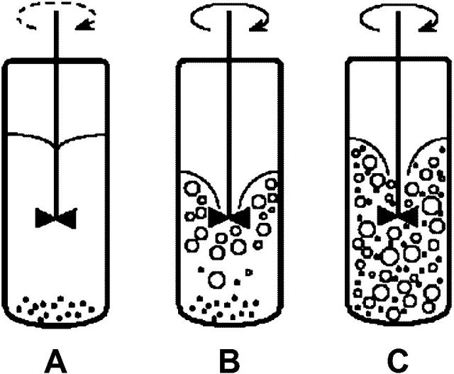
Another problem may be the deposition of the powdered catalyst at the bottom of the reaction vessel. We will show this on the example of a small laboratory autoclave with a centrally located stirrer.
However, even in a well-homogeneous reaction mixture, the main problem is to ensure a sufficient supply of hydrogen. We will now look at this issue in more detail.
Hydrogen transport problem
Hydrogenation is the reaction of an unsaturated substrate with hydrogen, which is almost always a deficient component. This is due to its very low solubility in the liquid phase. The solubility of hydrogen is (at normal pressure 1 atm and temperature 25 ° C), in ml of hydrogen gas per milliliter of solvent: in methanol 0.095, in ethanol 0.076, in cyclohexane 0.092, in benzene 0.071. Thus, in the case of hydrogenation at normal pressure, it is necessary to add to the solution every minute on the order of 0.5 ml of hydrogen per 1 ml of solution, in other words, to recover all the hydrogen in the reaction mixture about 5 times per minute.
The following figure gives a first insight into the issue of hydrogen transport:
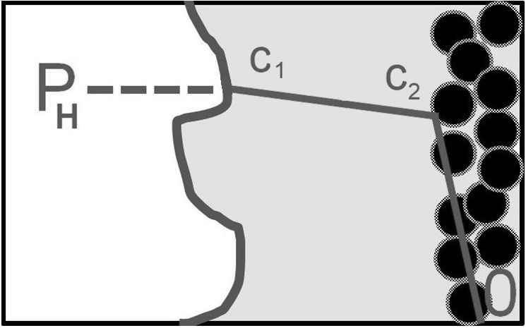
Hydrogen, whose partial pressure in the gas phase is PH, passes through the gas / liquid interface. The liquid at the interface is immediately saturated with hydrogen according to Henry’s law,
c1 = PH/H
where H is Henry’s constant. The hydrogen then travels through the liquid phase to the laminar film at the surface of the catalyst, where its concentration is c2. It reaches its own surface through the laminar film, where its concentration is cS; with this concentration it enters its own chemical process. From a practical point of view, it is advantageous to replace the concentrations in the liquid phase by „partial pressures“ in the liquid phase according to the relation
Pi = H∙ci [2.1]
The path of hydrogen to the catalyst surface is referred to as external diffusion. Before the hydrogen is consumed on the surface of the catalyst, it passes through the porous structure of the catalyst particles, which is referred to as internal diffusion; we will now address that.
Analogy between electrical conductivity, heat transfer and mass transfer
To discuss the phenomena of mass and heat transport, it is useful to define an analogy between these phenomena and electrical conductivity. This will allow us to use terms such as resistance or capacitance and their graphic symbols, as well as the laws applicable to the network of resistances and capacitances.
Table 2.1: Analogies of electricity, heat and mass transfer
| Phenomena | Electricity flow | Heat transport | Mass transport *) |
| Potential (voltage) | U – U0 | T – T0 | P – P0 |
| Current (flow) | I | rC | rD |
| Resistance | R | RC | RD |
| Conductivity | kR | kC | kD |
| (equivalence) | R = 1/kR | RC = 1/kC | RD = 1/kD |
| transmission rule | I = kR(E-E0) | rC = kC(T-T0) | rD = kD/P-P0) |
Internal diffusion
The previous table allows us to express the internal diffusion of hydrogen in the pores of the catalyst by the resistance to mass transfer, RD, while the mass transport rate is given by the relation rD=1/RD∙(P2-PS), where PS is the hydrogen concentration at the catalytic surface. For your own chemical reaction, if it is first order against hydrogen, it can be written
r = k∙PS = (1/RV)∙PS [2.2]
where
r local rate of hydrogenation
PS hydrogen activity at the catalytic surface
RV inverted value of the rate constant
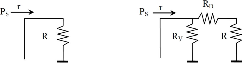
The RV and RD resistor symbols allow us to visualize the internal diffusion problem as follows:
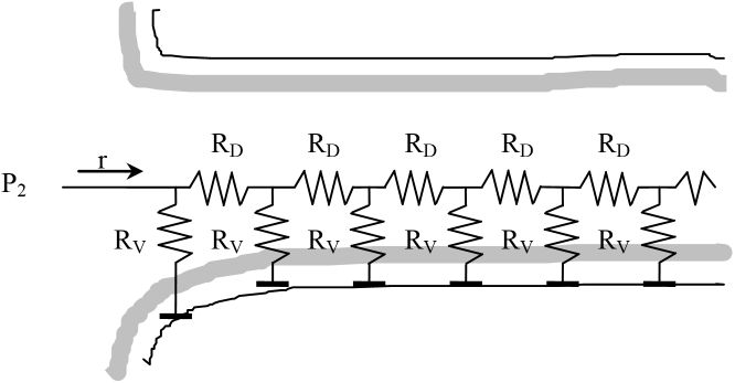
It shows how hydrogen progresses inside the pore while being consumed by a chemical reaction. This whole set of resistors can be expressed by a single resistor R, as shown in the following figure on the left. If it is an infinite network of resistors, then the total resistance R cannot change if we add another pair of resistors RV, RD (right) at the beginning of the network.
In the sense of Ohm’s law it is possible to write
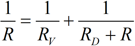
which will give
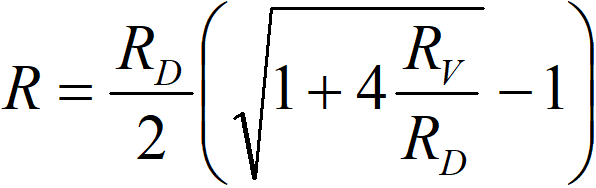
or if we prefer conductivities,
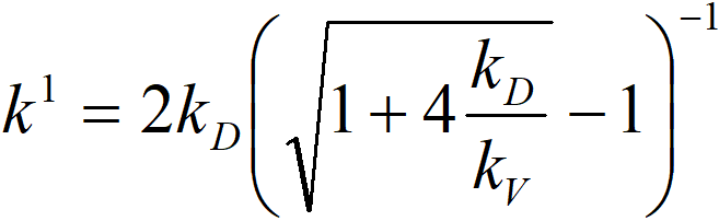
where
k1 observed rate constant
kV rate constant of a chemical reaction
kD diffusion constant
From the form of this equation, we can judge that quantifying the effect of internal diffusion will be very difficult – and this is the simplest case, namely a chemical reaction of the 1st order to hydrogen. It is therefore appropriate to perform experiments at different temperatures to determine the apparent activation energy. The activation energy of chemical reactions (temperature dependence of the constant kV) is of the order of 10 kcal∙mol-1, while the activation energy of diffusion processes (kD) is of the order of 2 kcal∙mol-1. A value somewhere in the middle of this interval indicates a problem with internal diffusion.
In kinetic measurements, practical measures are to be taken: to crush the catalyst into the smallest possible particles and then to keep them homogeneously dispersed throughout the volume of the reaction mixture. Let us mention here a catalyst that was once very popular, platinum black… with a density of 21 g/cm³. Such a catalyst does not remain dispersed, it always collects at the bottom of the reaction vessel. Fortunately, there is a wide selection of catalysts on the market with a much lower bulk density, supported catalysts. It consists of a fine and porous powder of activated carbon, kieselguhr or alumina, impregnated with a limited amount (1-5%) of active metal such as platinum, palladium, rhodium or others.
External diffusion
The intrinsic kinetics of hydrogenation, called „micro kinetics,“ is based on the term „hydrogen activity at the catalyst surface.“ Hydrogen must be supplied to the catalyst surface by mass transport to be consumed by the chemical reaction itself. If we denote the concentration of hydrogen at the surface of the catalyst cS and its solubility in the reaction mixture as cH0, then the rate of mass transport, RD, is given by Fick’s law,
rD = nD·(cH0 – cS) [2.6]
Seeing that the solubility of hydrogen in the reaction mixture is directly proportional to the partial pressure of hydrogen in the gas phase of the reactor, PH, this reaction can be written
rD = kD·(PH – PS) [2.7]
where
PH Partial pressure of hydrogen in the gas phase,
PS Effective hydrogen pressure at the catalyst surface,
kD Total mass transport coefficient.
The complex constant kD includes:
- The solubility of hydrogen in the reaction mixture (and its dependence on temperature.) Is expressed by Henry’s constant H:
cH0 = PH/H cS = PS/H - Diffusion coefficient (and its temperature dependence)
- Volume of liquid phase
- The amount of hydrogen gas bubbles in the reaction medium and, in general, the intensity of stirring of the liquid phase
The rate of the chemical reaction itself, r, can be written as
r = W·k(T)·f(PS, c,…) [2.8]
where
W amount of catalyst
k rate constant, which includes
- temperature dependence (Arrhenius‘ law)
- intrinsic activity of the catalyst
- proportionality constant
f (PS, c…) certain function, dependence on
- hydrogen partial pressure at the catalyst surface (PS),
- the concentration of the hydrogenated substance (c),
- concentration of other components of the reaction mixture
Under steady state conditions (which is certainly true due to the low solubility of hydrogen),
r = rD [2.9]
This equation opens the way to determine the hydrogen concentration at the catalytic surface, PS. If we add a really excessive dose of catalyst to the reaction mixture, then it can be assumed that r >> rD and PS → 0. The equation of real rate is then
r = kD·PH [2.10]
where
r real rate of hydrogenation, influenced by diffusion
kD diffusion constant
PH partial pressure of hydrogen in the gas phase
In this way, i.e. by hydrogenation with a large excess of catalyst, it is possible to determine the diffusion constant, which then serves to correct the effect of mass transport in kinetic measurements with a conventional catalyst dose. We will show a practical example later.
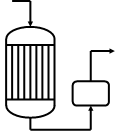
Autoclave for hydrogenation at elevated pressure
In Figure 2.1 we have already shown a simplified model of a reactor for heterogeneous hydrogenation. An example of the actual installation is shown in the following figure.
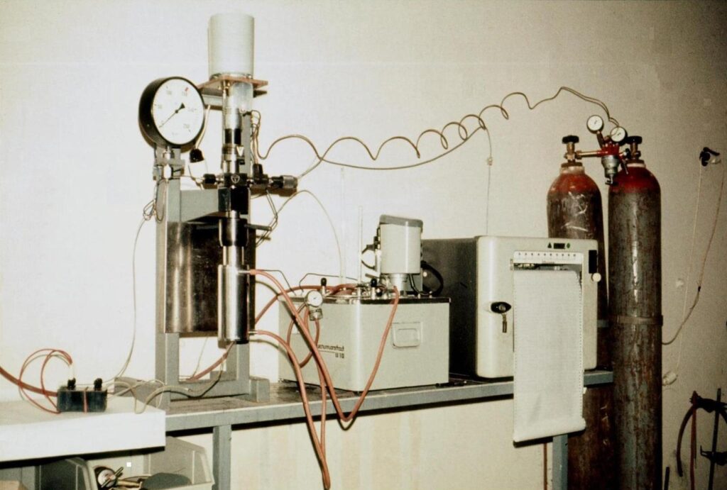
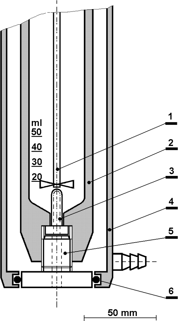
This autoclave is equipped with a double jacket for refrigerant circulation. The autoclave vessel is agitated by an axial stirrer with a magnetic head driven by a drive outside the pressure space. Hydrogen is supplied from the pressure vessel via a pressure regulator and via a valve. The photo is almost 50 years old, today DVM and a digital recorder are used to record the temperature.
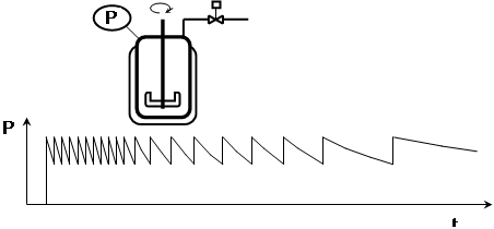
The vessel of our 200 ml autoclave is narrow and high, which is unfavorable for the homogenization of the reaction mixture. Different volumes of liquid phase and different stirrer speeds must be tested. Above all, it is necessary to achieve a rupture of the liquid level to saturate the volume with gas bubbles – dissolving hydrogen only across the liquid level would be absolutely insufficient. Another necessity is to homogenize the reaction mixture from the point of view of the catalyst so that the catalyst particles do not collect at the bottom, see Figure 2.1. The experimentally determined effect of the amount of liquid phase and stirrer speed is shown in Fig. 2.6.
Kinetic study:
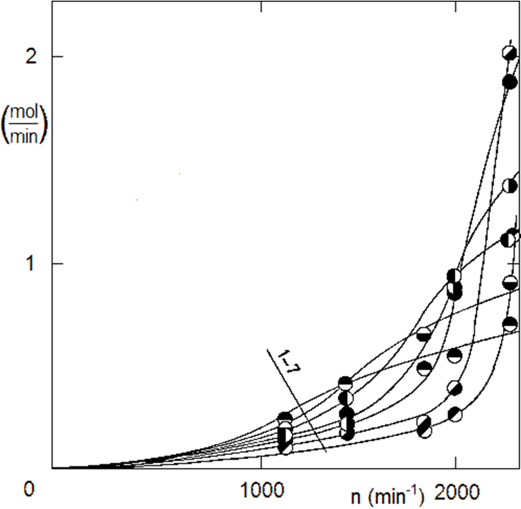
If the catalyst is overdosed, we notice a huge increase in hydrogen consumption as the agitator speed increases. It is therefore evident that the agitator speed needs to be increased to the maximum. The mixture should be whipped directly to create a real foam. Industrial autoclaves use various measures for this, for example, hydrogen is always fed directly under the stirrer – either via the hollow axis of the stirrer or via a side supply pipe. The gasification of industrial autoclaves is also aided by the installation in an autoclave vessel, such as a cooling coil. Returning to the laboratory autoclave: don’t be afraid to increase the agitator speed for fear of the agitator shaft bearing life. In fact, the rotating mass of the magnetic head stirrer assembly stabilizes the stirrer axis, just like a baby spinning top. It is at lower speeds that lateral throwing occurs, which reduces the bearing life. In the assembly in Figure 2.4, the original drive with the motor and pulley (with which the measurements were made according to Fig. 2.6) was replaced by a powerful asynchronous motor with a speed of 3000 min-1.
Monitoring the course of hydrogenation in the liquid phase
We start with a well-deserved catalytic duck, Fig. 2.7. It is a glass container with a double wall, the shell (here in the section) is tempered by a stream of liquid – heat exchanger. The duck is mounted on a shaker. This device looks outdated, but it can still be very useful, perhaps because it is made of glass, so if electrodes are installed inside, interesting things can be observed.
The reactor is connected to a burette system (here on the right they are on a reduced scale), burettes are used to measure the amount of hydrogen consumed.
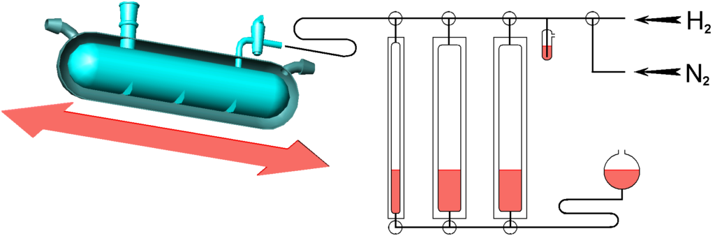
The liquid level in the burettes is adjusted manually by means of a movable expansion vessel. The fact that hydrogen is saturated by the tension of the buffer fluid can be a problem. However, there are also „dry“ variants with a cylinder and a piston.
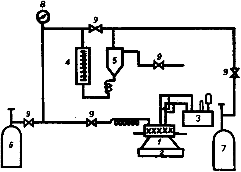
50 years ago, several Soviet laboratories tested the same system, of course made of steel and with armored burettes, for pressures up to 10 MPa (100 atm) – Fig. 2.8. In our opinion, they must have had a problem maintaining the temperature. For example, if the temperature of 400 K changes to 402 K at a pressure of 10 MPa, the pressure in the system changes (T1/T2 = P2/P1) by 0.5%, which represents a 5 m water column on the burette… Do not use!
With this control, it is easy to estimate when the batch should end; timely termination is good for selectivity as well as for the economy. The simple control system also has other functions, especially emergency shutdown by closing the hydrogen supply – in the absence of hydrogen, the reaction naturally stops.
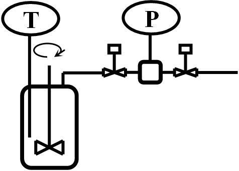
Variant: In one commercial laboratory autoclave, the measurement of the flow through a buffer vessel equipped with a manometer and two shut-off valves is described: during the alternating opening of the valves, the amount of hydrogen supplied can be calculated from the pressure drop in a buffer volume of known volume (Fig. 2.10.)
Another note on industrial practice: in the literature, it is sometimes recommended to carry out the hydrogenation with limited stirring. In such a mode, the apparent activation energy decreases and the system is easier to control. From an economic point of view, however, it does not make sense to use an expensive high-pressure autoclave if it is possible to work in a cheaper autoclave at a lower pressure, but with more efficient mixing. In addition, in general, any extension of the batch duration jeopardizes the selectivity of the process, reducing the yield.
Volumetric monitoring is not ideal for laboratory kinetic measurements. The pressure changes themselves are unsuitable for kinetic measurements, the main thing being that with each hydrogen addition, the temperature of the reaction mixture changes by a few tenths of a degree, which of course devalues the kinetic measurements.
Monitoring via heat balance
Hydrogenation is an exothermic reaction, so it is accompanied by the release of heat. A certain temperature gradient must be created to dissipate this heat. This temperature drop is proportional to the amount of heat released and thus to the rate of hydrogenation. If we can describe this phenomenon, we get a very natural means of monitoring the chemical reaction.
The heat balance and the temperature field in the autoclave system are very complicated. After all, for example, only the heat capacity of the steel shell of the autoclave is comparable to the heat capacity of the reaction mixture itself.
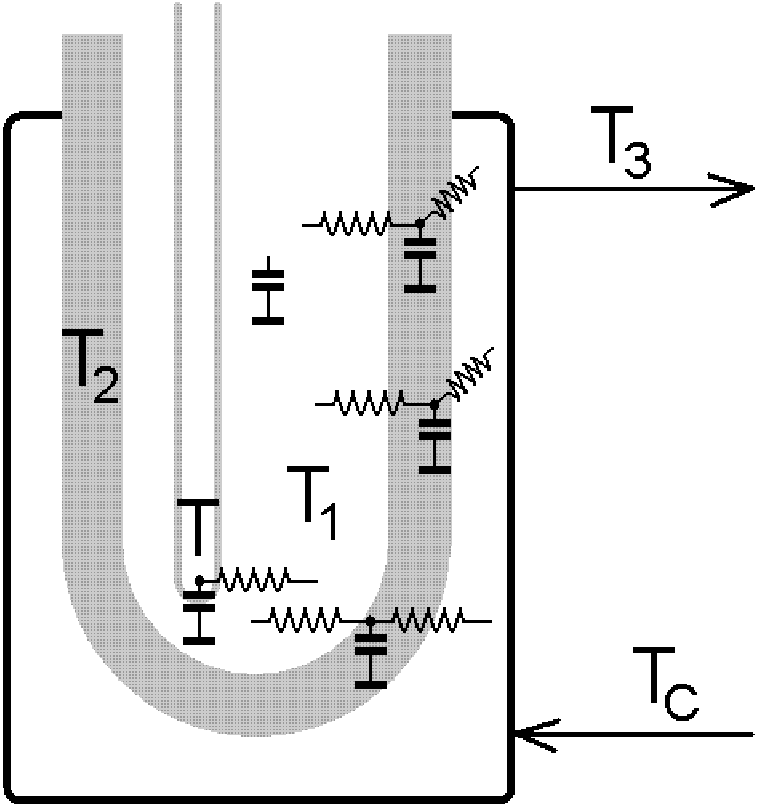
As our picture shows, heat transfer takes place through an endless network of capacitances and resistors. Nevertheless, simplifications can be made, for example taking T and T1 as identical and assuming that T2 is much closer to T1 than T3, in other words that the heat transfer resistance is concentrated at the interface between the autoclave vessel and the heat exchanger. Then it is possible to try to replace the whole system with a single capacity and a single resistor,

and create an extensive heat balance, ie a balance that includes the entire reaction system and the entire autoclave:
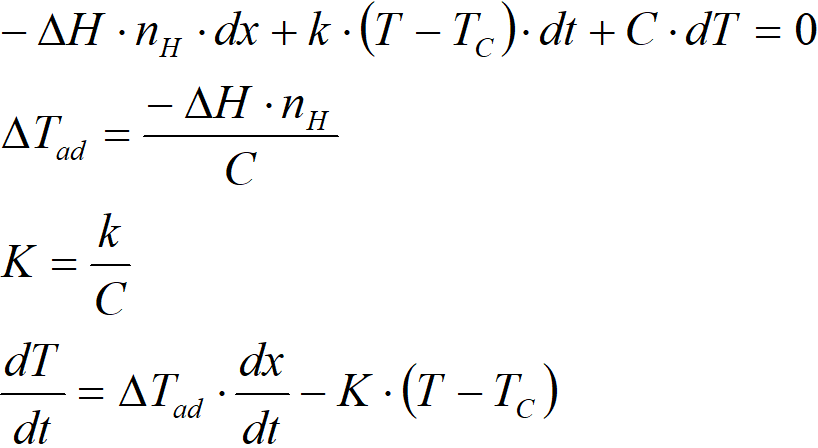
where
∆H molar enthalpy of the reaction, kJ∙mol-1
nH total hydrogen consumption, mol
x conversion
k total heat transfer coefficient, kJ∙K-1∙s-1
T temperature of the reaction mixture, K
TC heat exchanger temperature, K
t time, s
C heat capacity of the system, kJ∙K-1
∆Tad adiabatic temperature difference, K
K reactor cooling constant, s-1
k total heat transfer coefficient, kJ∙K-1∙s-1
For graphical presentation, it is advantageous to define the parameter „S“, whose dimension is K∙s∙mol-1
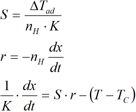
If dx/dt = 0, then the equation takes the form: S·r = T–TC. The product S·r thus expresses a steady temperature difference if the reaction proceeded for a sufficiently long time at a constant rate.
The heat balance [2.12] includes two constants, K and ∆Tad. These two constants are not independent of each other, they are connected via an integral of the heat balance,
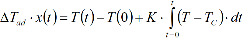
where
x(t) final conversion
T(t) final temperature
T(0) initial temperature (for x = 0)
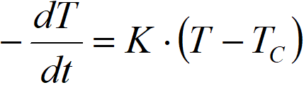
Thus, it is possible to calculate the constant ∆Tad based on the value of K. The value of K can be estimated experimentally by a simple experiment, when we let the reaction mixture temper without a catalyst (r = 0), ie
We create the initial temperature gradient, for example, by inserting a piece of dry ice (CO2) into a solution in an autoclave and then record the temperature response.
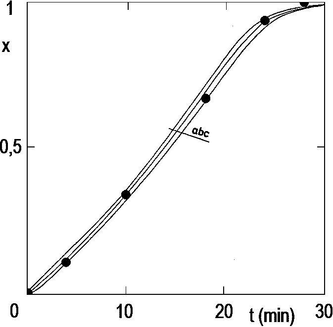
We will now verify our model by hydrogenation experiments. Figure 2.12 (see below) compares the conversions calculated by this model with GLC hydrogenation analyzes completed at different conversions.
The comparison confirms the suitability of the method. Even if we use a very inaccurate K value (the correct value for a stirrer speed of 2500 min-1 is 1.8 min-1), even then the calculated curves are very close to the results of direct GLC analysis. It is true, however, that the reaction proceeds at a virtually constant rate; the rates calculated at the beginning and end of the experiment, when temperature changes are more significant, are less convincing (see, for example, Figure 2.14 below).
We therefore state that heat balance is a simple and effective analytical method. We only had the problem that we measured the temperature difference with thermocouples that give only the order of 50 µV/K; therefore, even with state-of-the-art voltmeters, it is not possible to measure more accurately than 0.1 K. However, Pt100 sensors are now available on the market in miniature and, in conjunction with conventional industrial data acquisition systems, measure 100 times more accurately.
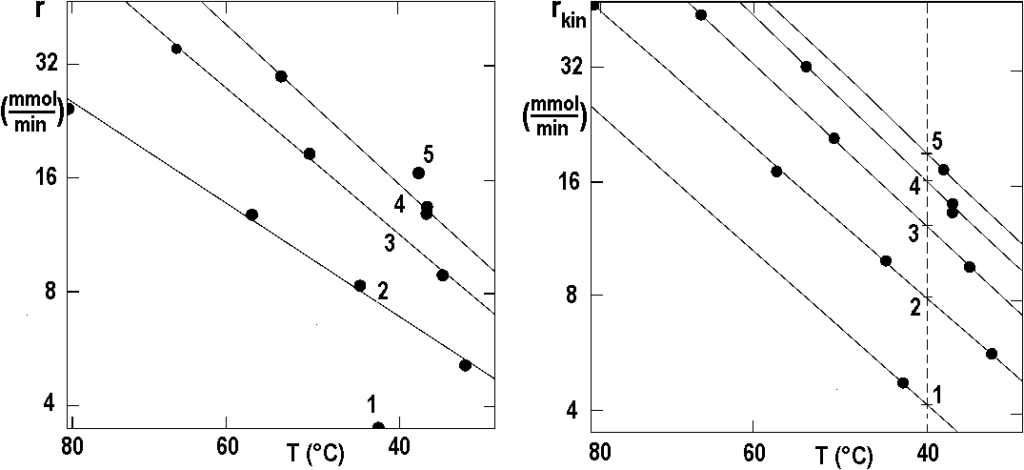
Figure 2.13 shows several velocity curves measured at different hydrogen pressures.
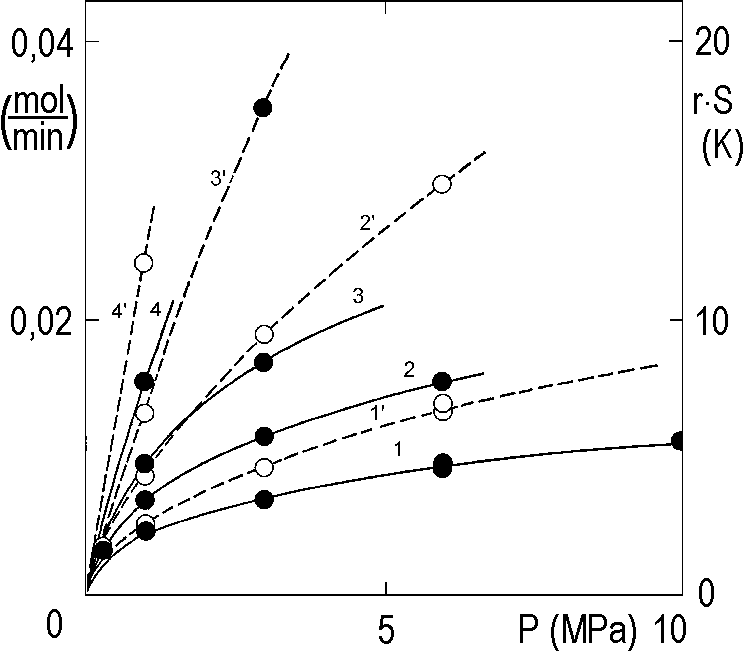
In the vertical axis on the right, the product r·S is plotted in this figure, which gives a picture of the heating of the reaction mixture during the experiment. The heat released increases the temperature, under certain conditions, by almost 20 K. The general rule is that increasing the temperature by every 10 K doubles the speed. Thus, the curves plotted in Figure 2.13 in dashed lines offer no idea of the kinetics at constant temperature.
In the next paragraph, we propose a method for correcting data loaded due to external mass and heat transfer. The output is then isothermal kinetic data. The method is not completely universal, but it has the advantage that it is very instructive.
Procedure for elimination of external mass and heat transfers
The experimental data that we will further process are extensive (related to the whole system) and therefore it is necessary to observe a constant volume of the reaction mixture and constant external parameters in the whole series of experiments. This is a study of the hydrogenation of nitrobenzene (10 ml nitrobenzene in 30 ml ethanol) on a 3% Pd/C catalyst (100 mg) under elevated hydrogen pressure under conditions where the external heat and mass transfer is not negligible. We start with equation [2.7] (see above),
rD = kD·(PH – PS) [2.7]
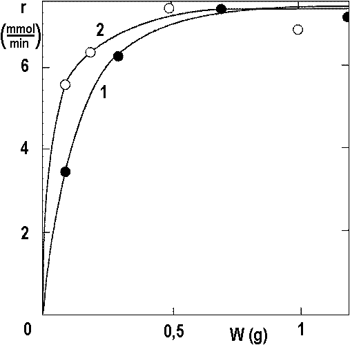
To determine the value of the total hydrogen transport coefficient kD, we perform a series of measurements at relatively low pressure and with a large excess of catalyst.
Figure 2.14 shows the course of several experiments with an increased amount of catalyst. The conversion curves were calculated from the temperature curves as described above. Ignore their course at too low or too high conversions, in these areas the numerical derivation fails due to sudden changes in temperature. We observe here that at a relatively low catalyst dose, i.e. under kinetic conditions, the reaction is practically 0 order to the hydrogenated substance. However, there is an interesting paradox, at excessive catalyst doses, ie under diffusion conditions, the rate of conversion decreases somewhat. Here is a change in the solubility of hydrogen in the reaction mixture with continued conversion (Pi = H∙ci, where as shown here, the Henry’s constant depends on the composition of the reaction mixture). The solid points show the solubilities of hydrogen measured by an independent method in model mixtures, but at lower temperatures.
Solid lines – hydrogenation rate (r) as a function of conversion at 40 ° C, 0.29 MPa.
Catalyst amount (g): 1 – 0.1; 2 – 0.3; 3 – 0.7; 4 – 1.2.
In the following, we will discuss only the conversion rates x = 0.5. Figure 2.15 shows the experiments in Figure 2.14 and still other experiments.
Temperature TC: ● 1 – 40 ° C, ○ 2 – 70 ° C.
The data from Figure 2.15 allow estimating the value of ND: if PS → 0, we get
ND = RD/P
In Figure 2.13 we showed the rate of hydrogenation as a function of pressure, but the measured curves (empty dots) were affected by the external mass and heat transfer to the extent that they had no telling power. It is essential to clean them from the effects of transport phenomena. Again, the following method is far from universal, but very instructive.
The correction requires accepting the hypothesis of the shape of the reaction rate. The most sensible thing is to choose the power dependence,
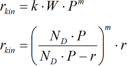
This equation is the basis of an iterative algorithm, where the first estimate of m is performed and then the first estimate of the value of the activation energy is obtained.
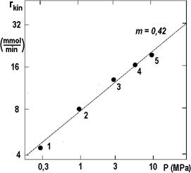
The following figure 2.16 shows, in Arrhenius coordinates, two sets of data from figure 2.15 – measured values on the left, corrected values on the right. The curves in the left figure are not parallel, while the lines on the right, an estimate based on equation [2.16], are already almost parallel.
The isothermal points from Figure 2.16 are shown in the following Figure 2.17 as a function of pressure in logarithmic coordinates. The slope of the connector is 0.42; with this value, the iteration can be repeated.
The result of all these efforts has already been shown in Figure 2.13: there are measured curves (empty points, dashed lines) and corrected curves (solid points, solid lines) for temperatures TC, (°C): 1 – 30; 2 – 40; 3 – 50; 4 – 70.
Adjusting the results by „weighing“
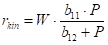
Due to the limited range of experimental results, it is advisable to group all results into a single curve. Temperatures are converted to a single temperature, for example to T0 = 40 °C. Furthermore, it is good not to over-trust the points that required large corrections for mass transport. It is therefore appropriate to proceed to a certain weighting, we have chosen
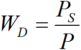
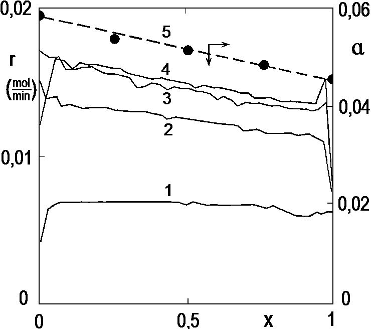
Figure 2.18 takes over all the points from Figure 2.13, converted to temperature T0 = 40 °C (empty points). These points were averaged with WD weights, which gave full points. We experimentally interpolated the curves corresponding to four different models using the following regression method:
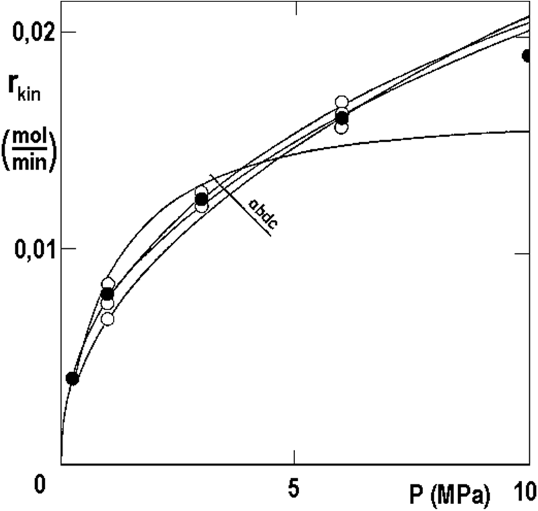
Each model in Figure 2.18 corresponds to some idea of hydrogenation control step, for example for (a) the rate is determined by hydrogen adsorption in molecular form H2, model (b) corresponds to the idea of hydrogen adsorption in atomic form H, (c) is the same for very low surface coverage, (d) is the power dependence for m = 0.42.
Interpretation of experimental results
It is said that if the model has three or four parameters, it is already possible to model an elephant. Many discussions end with this statement …
Returning to serious considerations, Figure 2.18 shows that it is always possible to interpolate experimental data with a curve, but that it is not always possible to decide which model is correct if a sufficient amount of experimental data is not available. In this case, it would be desirable to measure at one even higher pressure, but we did not get to that then…
More generally about the reproducibility of measurements in catalytic hydrogenation. If you want to achieve a series of coherent kinetic measurements, you must pay special attention to the measurements, which may seem exaggerated. Thus, for a whole series of experiments, it is necessary to use hydrogen from a single pressure vessel. Reserve excess catalyst and especially avoid freshly prepared catalyst. Shake the powdered catalyst vial well before use. Someone insists on a hydrogenated substance freshly prepared, but if you distill the hydrogenated substance every morning, you will never achieve coherent results from hydrogenation experiments. The correct procedure here is to distill only once and to store the substance to be hydrogenated under nitrogen in precise portions (for example, 25 ml) in sealed ampoules or vials closed with Teflon. In each experiment, the entire contents of the vial are poured into the reactor – the dosage can be controlled by differential weighing of the full and empty vials. We have already mentioned the problem of humidity; it can be prevented by using a polar solvent, in the experiments discussed above 25% by volume of nitrobenzene in ethanol was used. A series of preliminary experiments is required to master the experimental technique. So we need to do something to achieve „presentable“ results, as the French say.
3. Hydrogenation in the gas phase
Catalyst bed
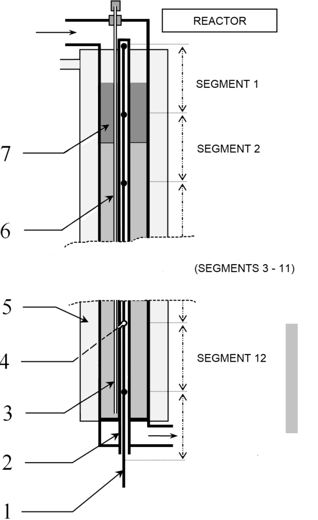
In the previous chapter, we were dealing with a heterogeneous catalyst in the form of a fine powder. The purpose of the crushing was to obtain the largest possible catalytic surface area from a given amount of catalytic mass. However, sometimes it is more advantageous to use a compact bed of catalytic tablets. The typical arrangement is then twofold:
a) Under a hydrogen atmosphere, the catalyst tablets are sprayed with the reaction mixture in the liquid phase, the gas proceeding either in cocurrent or countercurrent. This method is used, for example, in the food industry – hardening of vegetable fats, conversion of fructose to sorbitol, etc.
b) A hydrogen-containing gas saturated with a hydrogenated substance passes through a bed of pellets of catalyst.
Hydrogenation reactions generally release a significant amount of heat, which must be removed. For example, it is possible to divide the catalyst into several sections, between which there are cooling sections, or to insert cooling coils directly into the catalyst bed. As a rule, it is best to use a tubular reactor – the catalyst is in the tubes, the coolant circulates in the inter-tube space.
Liquid phase processes require an even distribution of liquid over the entire surface of the catalyst bed. The problem with the gaseous reaction mixture is less significant, however, I remember one unusual situation. It was a hydrogenation in a tubular reactor, which was supplemented at the outlet with a simple vessel filled with catalyst in order to react any residual substrate, Fig. 3.1.
In our case, the interconnection of the reactors was realized by a pipe, which resulted directly in the bottom of the adiabatic reactor, a simple vessel filled with catalyst tablets. The diameter of the connecting pipe was chosen according to the practices that prescribe a linear velocity between 15 and 30 m∙s-1 for the transport of the gas phase. One day, while inspecting the adiabatic reactor, we found that it was completely empty. The gas stream managed to lift the layer of catalyst pellets and bring them into a fluid state, so that they flew away. This story reminds us that there are also fluidized bed reactors that are used, for example, to produce aniline in Brazil.
We will focus on our tubular catalytic bed reactor. The basic requirement is the mechanical stability of the catalyst pellets. The disintegration of the pellets means an increase in the pressure drop only after the reactor is clogged. The reaction takes place at active centers on the surface of the catalyst and therefore a huge surface area, up to a few square meters of surface area per gram of catalyst, is desirable. Thus, the structures are very porous and a priori, the strength of such pellet is limited.
The catalyst is manufactured by the following basic processes:
1) Impregnation of the support with an active metal solution. Platinum metals are expensive, in which case a porous ceramic support is naturally taken and impregnated with a metal salt. The mechanical stability of the ceramic support is very good, examples being catalytic inserts in car exhausts.
2) Precipitation of a mixture of chemical solutions and compression of this mass into pellets. This is followed by firing, which releases gases, and the process is a bit like burning lime. The product is sufficiently porous, but the strength is often insufficient. A suitable compromise must be found between mechanical stability and catalytic activity. Hydrogenation catalysts often require chemical reduction before use; in this case, the last stage of production after reduction is passivation, which facilitates transport and handling at the point of use.
3) Another story concerning the production of aniline. Ranney nickel is often used in liquid phase hydrogenations, a commercial catalyst in the form of a fine powder is produced by leaching an alloy of nickel and aluminum (2 Al + 2 NaOH + 6 H2O → 2 Na[Al(OH)4] + 3 H2). Since a large amount of heat is released during the production of aniline in the gas phase, it was interesting to try to use Ranney’s Cu/Al alloy leached on the surface as a grain catalyst, as the metal alloy is a very good heat conductor. It was a complete failure, within a few tens of hours in the reactor there was a complete deactivation of the catalyst, probably due to a change in the grain structure (creep).
We conclude that the main parameters of the catalyst bed are: activity, selectivity, longevity – this is given by both chemical and mechanical stability, because an excessive increase in bed pressure loss will cause the need for premature catalyst replacement. Any change in regime is detrimental to the mechanical stability of the bed: sudden changes in temperature (especially at the beginning of the hydrogenation cycle), downtime, etc. The life of the bed is also affected by the quality of the raw material in terms of impurities such as sulfur content in the supplied hydrogen, etc.
Let us also mention the problem of catalytic bed inhomogeneity. The following picture shows a part of the tubesheet of an industrial reactor, where hundreds of tubes open. At the end of the catalytic cycle, when the reactor lid is removed, a contraction of the depleted catalyst is noted, which, however, differs from tube to tube. In addition, the individual pipes differ greatly in terms of pressure loss (measurement method: when a gas of constant flow is introduced into the pipe, then the pressure loss is characterized by the value of the overpressure at the inlet). This problem has its origins in the production of catalyst, which takes place in small batches, so in the supply of catalyst, each barrel has its own history. The tubes are filled through a funnel with a shank of smaller diameter so that no empty „holes“ remain in the catalyst bed. Even better, however, is to use a template with holes smaller than the mouth of the tubes; in addition, the catalyst from several barrels is naturally mixed during filling.

Test equipment for gas phase hydrogenation
We will focus on the development of an industrial process for the production of aniline. In our country, aniline is industrially produced in the gas phase; a reaction mixture of hydrogen saturated with nitrobenzene vapor is passed to the catalyst bed. Aniline is formed by reaction
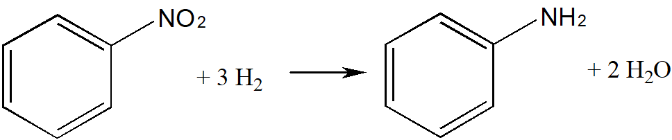
Industrial production takes place at the reactor assembly according to the following scheme:
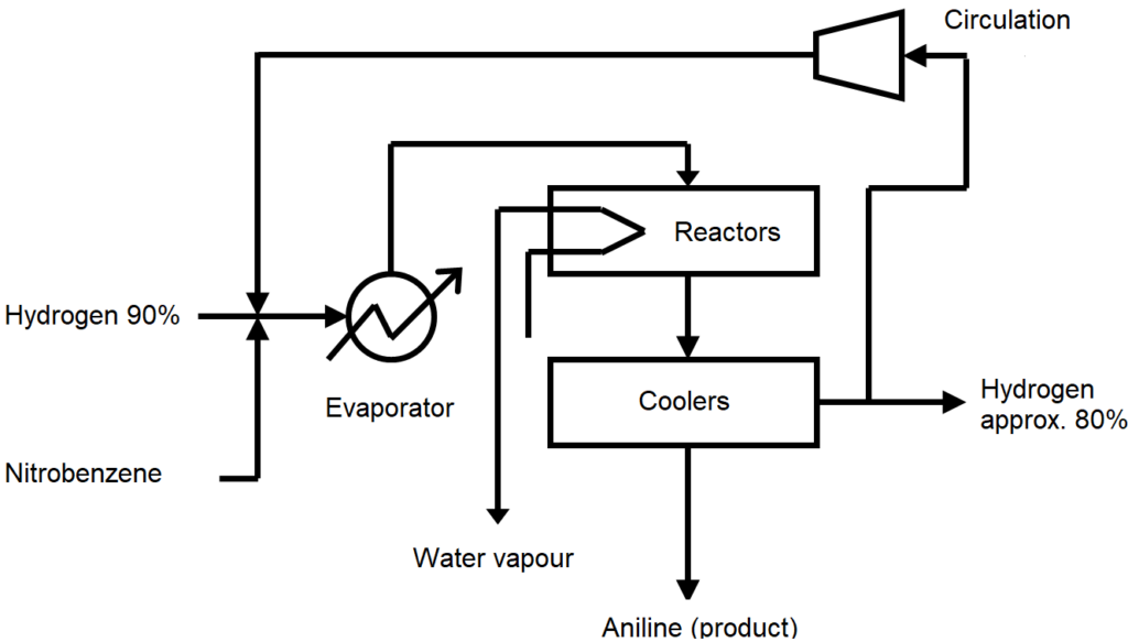
The industrial reactor is tubular and is supplemented by an adiabatic reactor, see Figure 3.1. The catalyst is in the form of cylindrical tablets of the order of 5×5 mm. The heat of reaction is removed by steam in the inter-tube space of the tubular reactor, so that enough heat is obtained for the distillation of the crude product, which is one of the advantages of gas phase technology. In the following text, we will use the term „catalytic cycle“, which means the period of use of the catalytic bed until its replacement.
Aniline is a commodity. The quality of the product must be flawless, but to succeed in the market it is necessary to succeed in the field of production costs. This is mainly influenced by two parameters:
(1) Since the removal of traces of raw material from the crude aniline is expensive, the hydrogenation cycle must be completed when the first traces of nitrobenzene appear at the outlet of the reactor unit. Catalyst replacement must follow, which burdens the economy (loss of production time, catalyst price, logistics, ecology, etc.).
(2) The cost of hydrogen circulation, which depends on the pressure drop of the reactor, is a fairly important item of production costs. Before a mechanically stable catalyst could be found, the catalyst pellets tended to disintegrate and it was often necessary to terminate the catalytic cycle prematurely, i.e. before the penetration of nitrobenzene, due to complete clogging of the reactor tubes.
We therefore selected a suitable catalyst and optimized the operating parameters on our test facility. These were 23 test catalytic cycles lasting from 200 to 1700 hours.
The test equipment is shown in Figure 3.4. For the research of the process, a tubular reactor with a single tube was installed, on which there is a coaxial jacket with boiling water. It boils water at a controlled pressure, ie at a constant temperature. Note that to ensure the supply and circulation of liquid water, steam is supplied, which is partially liquefied in the condenser.
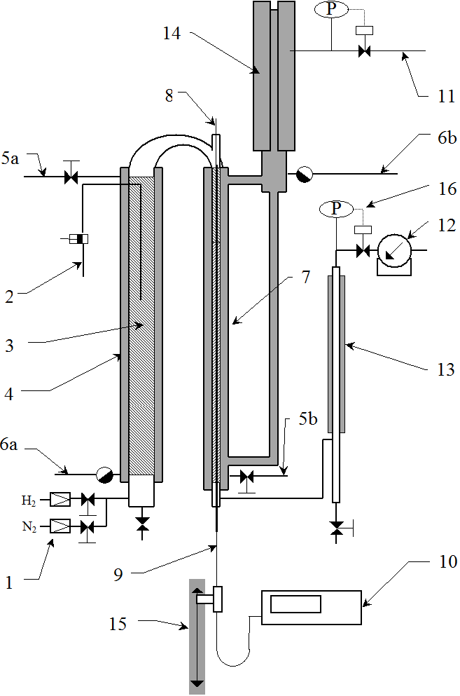
A detailed view of the reactor is shown in Figure 3.5. In the axis of the reactor is a probe for measuring temperature. The probe contains a bundle of twelve thermocouples at regular intervals.
Some 150 thermocouples would be needed to measure the entire axial temperature profile, which is practically impossible to implement. It is also possible to use a single thermocouple and move it step by step, which in turn takes too long, because the measurement requires waiting at least 30 seconds at each point, the whole would take about 75 minutes.
The trick of temperature measurement is to install 12 thermocouples at a distance of 30 cm from each other and to move them simultaneously with a step of 2 cm on a path of 30 cm. All 12 temperatures are measured simultaneously, so the total measurement time is 15×30 seconds, ie acceptable 7-8 minutes. Note that the thermocouple in its 16th position is in the 1st position of the next thermocouple, so they control each other’s function. The beam consists of sheathed thermocouples with an outer diameter of 0.5 mm, so that the beam can be moved already in a probe with a diameter of 3 mm. The experiments presented below were undertaken with a 10×1 probe, ie with an inner diameter of 8 mm.
Our sampling system also deserves attention. As we will describe later, we use a temperature profile to determine the concentration profile along the entire length of the reactor, but is this procedure correct? To verify it, it is necessary to take samples along the entire length of the catalyst bed. Naturally, sampling valves can be installed along the entire length of the pipe, but such branches inside the pressure jacket are technically extremely difficult. We installed a capillary in the catalytic bed along the temperature probe, which emerges from the reactor head through a seal. The capillary had an outer diameter of only 1 mm. When this capillary is extended step by step, it is possible to take samples of the reaction mixture along the entire length of the bed. Of course, once the capillary is withdrawn, it cannot be returned to its original position – but by repeating this with each reaction cycle, we have obtained a sufficient database to verify the temperature profile – in addition to further knowledge on by-product formation, etc.
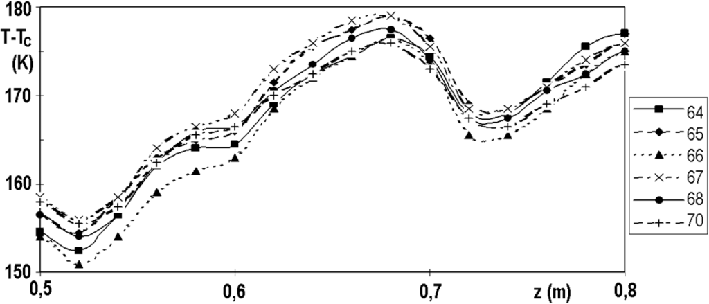
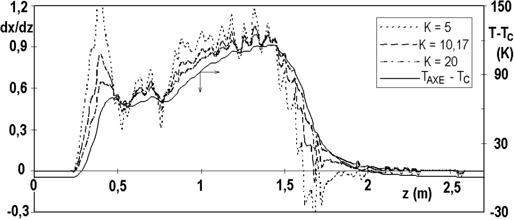
The temperature profile, which is short and sharp at the beginning of the hydrogenation cycle, decreases and lengthens over time – see Figure 3.6. In all figures, the profiles are identified by operating hours, for example „25“ means 25 hours from the start of nitrobenzene dosing. From this figure we can see that, for example, the catalyst at the 1.5 m coordinate does not start to work until after a hundred hours, and even at 300 hours the reaction takes place on the first 2 m of the catalyst bed. When the profile reaches the end of the bed (here: coordinates 2.7 m), we observe a massive penetration of nitrobenzene at the outlet of the reactor, the catalyst bed is depleted and needs to be replaced. In industrial practice, monitoring the axial profile of temperatures is a method of prediction.
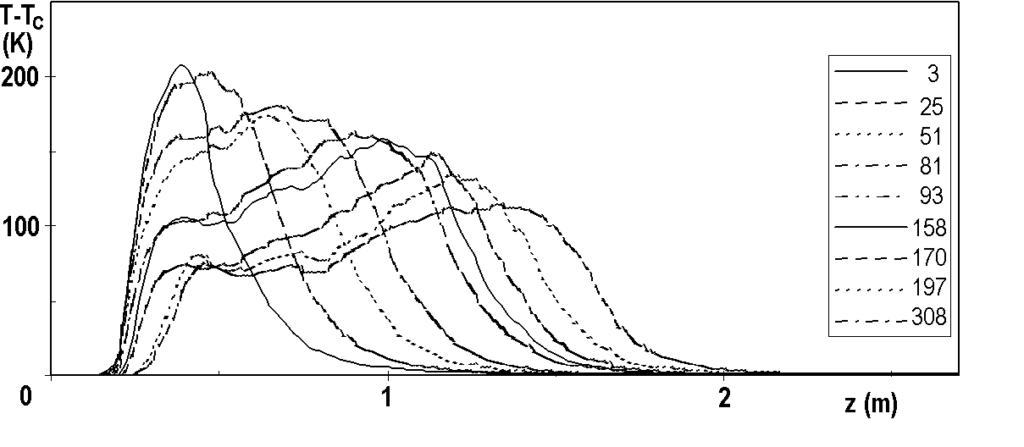
Note: Why doesn’t the profile start at coordinate 0? The coordinate 0.00 corresponds to the level of the catalyst in the freshly filled tube, i.e. before the reduction. During the reduction and partly during the hydrogenation cycle, the catalyst becomes more compact. The tubular reactor is vertical, the lower end of the bed is fixed, so the beginning of the catalytic bed is shifted.
The temperature profile has a fine structure or small fluctuations, which are perfectly reproducible. Figure 3.7 shows several profiles measured over a relatively short period of time and Figure 3.8 shows the same, but in detail. The reproducibility of the measurement is surprising when we realize that the thermocouples slide freely in the probe with a diameter of 8 mm and their ends are not forced to come into direct contact with the inner wall of the probe.
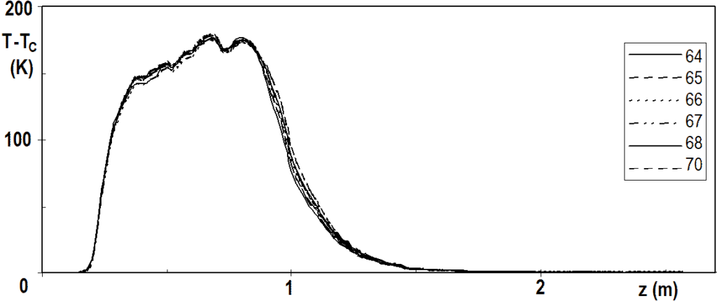
Cycle No. 20, operating hours noted in the legend.
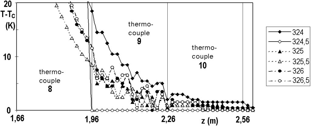
t is not right to confuse the fine structure of the temperature profile, perfectly reproducible, with the technical problems of measurement. For comparison, we show in Figure 3.9 the difficulties that caused us for some time the failure of thermocouple No. 9. The measurement fluctuations were random, chaotic. The cause of the problem was a loose screw on the terminal block, not the thermocouple.
Heat balance
The calculation of the heat balance in a tubular reactor with a catalytic bed was proposed as an analytical method by K. Wilson, 1949. As we will see, the method is very similar to the procedure we described in the chapter on hydrogenation in an autoclave.
If we take a short length of catalytic bed, then the heat balance consists of three members:
– change of enthalpy of reaction current between output and input, G·cp·dT/ dz
– heat released by a chemical reaction
– heat dissipated to the heat exchanger, U·(T-TC),
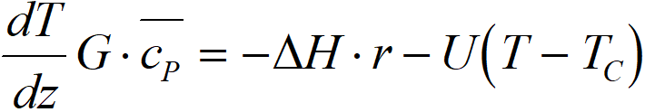
TC heat exchanger temperature [K]
G mass flow per unit cross section, mol.s-1m-2
cp mean heat capacity, kJ·mol-1K-1
ΔH reaction enthalpy, kJ·mol-1
r hydrogenation rate, mol·s-1m-3
U heat transfer coefficient, kJ·s-1K-1m-3
n0 flow of nitrobenzene per unit cross-section of the bed, mol.s-1m-2
x degree of conversion
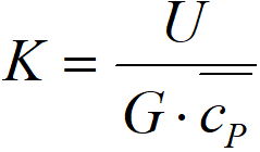
Then we can define two complex constants,
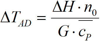
ΔTAD adiabatic temperature difference, K
K cooling constant, m-1
By further modifications we get to the heat balance in the form of a completely simple equation,
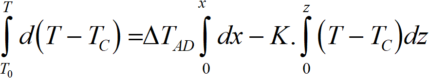
from which we get integration
T temperature at coordinate z, K
x degree of conversion at coordinate z
z length coordinate of the bed, m
We will now deal with the constants ΔTAD and K. For simplicity, we take x = 1 and also the zero value of the first integral of equation [3.8]. This is how we get to the equation with three parameters:
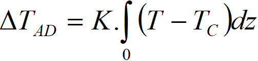
We estimate the value of K, for example, from the course of temperature stabilization in the layer of inert Raschigs, in our case the estimate is about K = 10 m-1. Let’s look again at the effect of the uncertainty in the value of the cooling constant K on the hydrogenation rate profile – we compare the calculation with this value with the calculation with the value K half, resp. double. For all three values, the middle part of the hydrogenation rate curve is very similar – Figure 3.10.
An incorrect K value only affects the area where the temperature changes significantly – negative speeds can even occur at the end of the profile.
The calculation of hydrogenation rate from the temperature profile is subject to considerable fluctuations, which is due to the fine structure of the temperature profile (see Fig. 3.8). It is therefore reasonable to proceed with the numerical smoothing of the velocity curves – see below.
Conclusion: based on the axial temperature profile, it is possible to calculate the velocity profile and especially the concentration profile. The values are most reliable where there are no large temperature changes, i.e. in the middle part of the temperature profile.
Calculation method
The hydrogenation rate profile from Figure 3.10 was created by simple differentiation. If we denote t[i] the field of temperature differences T – TC, where i is from point N° 1 to point N° 136 (in the case of a profile with a length of 2.7 m) and r[i] the field of values dx/dz,
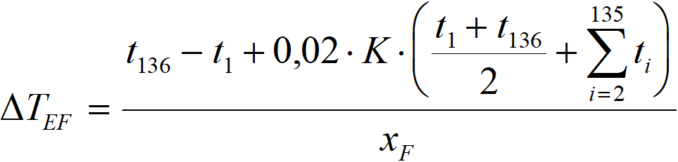

ΔTEF effective value ΔTAD, used in the calculation
When we compare the temperature curve with the curves of the calculated velocities in Fig. 3.10, then we state that the velocity curves are very „scattered“. Taylor smoothing formulas could be used to smooth the curve, we consider it better to interpolate the conversion curves at individual points with a straight line, thus obtaining the velocity (straight line direction). Numerical processing consists in least squares interpolation of a straight line over a section of ± 5 points from a given point, using weighing:
Thus, we „beautified“ the dx/dz curves by smoothing without limiting their explanatory power. In the next we will focus only on conversion curves. We will return to hydrogenation rate curves only in the next chapter.
Example of application
Thus, we learned to calculate the conversion increment, Δx at each moment and on each section of the catalytic bed. When we multiply this value by the amount of injected nitrobenzene nNB (kg∙h-1), we get the amount of nitrobenzene processed per hour on a given section of bed. By summing over time, it is possible to determine the amount of processed nitrobenzene in a given section from the beginning of the hydrogenation cycle. Figure 3.11a shows such curves for hydrogenation cycles Nos. 20-22. The total amount of nitrobenzene processed per hour represents the entire area under the respective curve.
The following figure is a generalization of these curves.
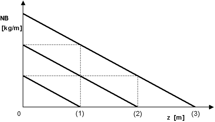
We display idealized waveforms here as parallels under a certain slope. When the profile reaches point (1), the amount of nitrobenzene processed per hour represents the area of the triangle below the first line. Over time, the profile reaches point (2), the amount of nitrobenzene processed being four times. When the reaction reaches point (3), 9 times more nitrobenzene has already been processed. The lifetime or usability of the catalyst bed is therefore not a linear function of the bed length, but rather the square of the bed length. One old French patent proposes the production of aniline in two tubular reactors in series. Thus, if the capacity of two reactors in series is exhausted, the second reactor is placed at the head and the first reactor, after replacing the spent catalyst with fresh one, is placed second in the series:

In this way, the catalytic mass is better utilized. In addition, since the fresh nitrobenzene stream never comes into contact with the fresh catalyst, extreme temperatures do not occur in the first hours of the catalytic cycle and it is possible to operate at full load from the beginning without compromising the mechanical stability of the tablets. However, an industrial process operated in our country (and licensed abroad) does not use this arrangement.
4. Kinetics of „gas phase“ hydrogenation
For the moment, we will ignore the parentheses we used for the term „in the gas phase“ and focus on determining the rate equation of this hydrogenation. The aim is to find a means for determining the axial activity profile of the catalyst, which will then make it possible to model the course of deactivation during the hydrogenation cycle.
The experimental procedure for determining the kinetics consists in changing the process parameters: injection, gas / nitrobenzene molar ratio, temperature, pressure, hydrogen concentration in a mixture of hydrogen and nitrogen. During the catalytic cycle, after several tens of hours, when the mode stabilizes, we proceed to changes in the parameters and after a certain time (1.5 hours) we record the temperature profiles with an interval of 30 minutes. Such a series of short-term experiments, each lasting a total of 2 hours, is shown in Table 4.1.
Table 4.1: Short-term experiments during cycle No. 20, hours 312 – 326
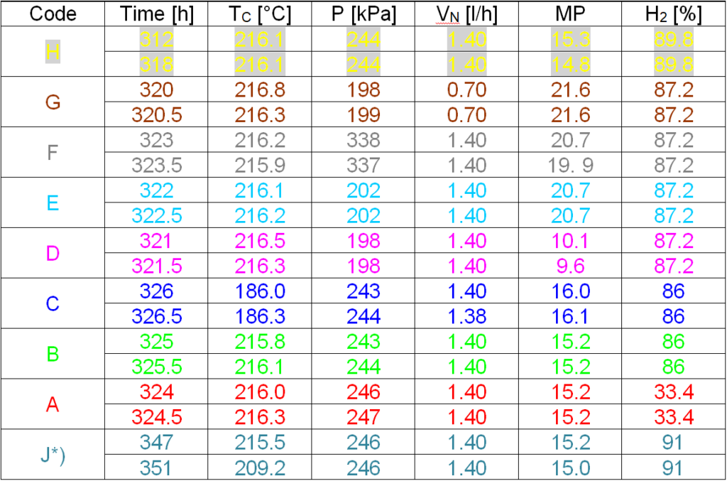
MP Molar ratio of gases to nitrobenzene at the reactor inlet
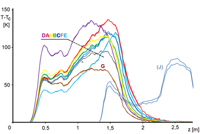
The temperature profiles measured during the short-term experiments in Table 4.1 are shown in Figure 4.1.
We reiterate our goal: since we can already calculate the hydrogenation rate profile based on the temperature profile, we will try to determine the decrease in the activity profile over time. The simplest is to try to determine the activity as a rate constant in the type equation
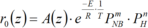
r0(z) reaction rate at the z coordinate, mol∙m-3s-1
A(z) activity of the catalyst at the z coordinate
E/R apparent activation energy vs. gas constant
m order of reaction with nitrobenzene
n order of reaction with hydrogen
One of my colleagues once published a result:
Pexidr V., Heral V., Chemical Industry 33, 229 (1983).
The equation was
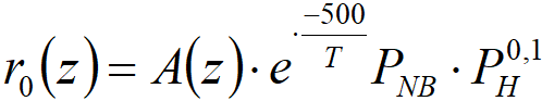
In order not to repeat the measurements already published, we will show here the application of equation [4.2] to newer measurements, ie the series from Figure 4.1.
In Figure 4.3, we cut the curves at a conversion of 0.9, because the activity curves become too uncertain for higher conversion – we note a miraculous increase in activity towards the end of the profile. But this is obviously impossible. In addition, we performed this experiment: we removed the initial part of the catalyst bed to give the reaction mixture a fresh catalyst – see Figure 4.1, curve [J]. We state that although the section of the reactor behind the coordinate 1.5 has not yet processed practically any nitrobenzene, the catalytic charge is already considerably deactivated here. We assume that in this region, where temperatures are relatively low, by-products formed in the reaction zone settle and that these impurities are in the form of a viscous liquid. It is quite possible that these impurities proceed by a mechanism similar to GLC chromatography.
Thus, in the case of nitrobenzene hydrogenation, we have a true „stationary“ liquid phase that limits the access of reactants to and from the surface. So even when it comes to „gas phase hydrogenation“, the reaction actually takes place through a liquid film. Note also the ratio E/R = 500 in equation [4.2]; such a value is typical for mass transfer, while the activation energy of the chemical reaction itself must be of the order of E/R = 5000 (so, 10 kcal∙mol-1). We performed 6 series of short-term experiments during two catalytic cycles (HC20 and HC21) and the result was always the same: the dependence of the hydrogenation rate on temperature is practically negligible.
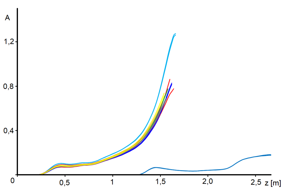
A detailed analysis of our temperature curves also provides some evidence of the existence of that laminar film – probably associated with the term „capillary condensation“. Figure 4.4 shows the hydrogenation rate at z = 1 m as a function of time for our series of measurements:
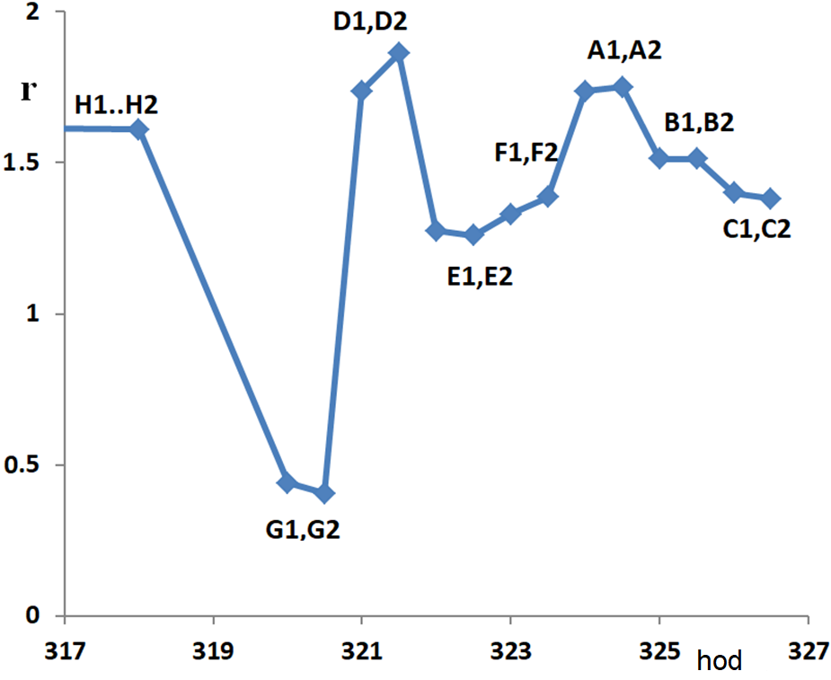
Take, for example, point G2, hour 320.5. After measuring the temperature profile G2 and changing the parameters, measurement D1 was performed after 90 minutes and measurement D2 after another 30 minutes. We see that between the 90th and 120th minute after the change of parameters, the speed still changes in the direction of the change, in other words, the establishment of a new equilibrium on the surface is not finished two hours after the change of parameters.
According to our findings, the rate of hydrogenation of nitrobenzene in the gas phase is practically independent of temperature and hydrogen pressure. It is proportional to the partial pressure of nitrobenzene or indirectly proportional to the partial pressure of hydrogenation products (water, aniline). The reaction proceeds through a liquid film.
In conclusion
This text was devoted to the theory and practice of heterogeneous hydrogenation. If we managed to at least partially get rid of this mystery, then our work served its purpose.
Abbreviations and symbols
A(z) catalyst activity at z coordinate
aR olefin activity on the catalytic surface
aH atomic hydrogen activity on the catalytic surface